Authoring Manuscripts

Overview

On this page, we’ll show you how to author an academic manuscript with Quarto in Jupyter Lab. You’ll learn how to:

• Preview your manuscript using Jupyter Lab.

• Add scholarly front matter to describe your article.

• Add figures, tables, cross references, and citations with Quarto-specific markdown.

• Include output from computations using inline code or embedded from external notebooks.

The commands and syntax you’ll learn will apply to any tool you might use to edit notebooks, not just Jupyter Lab. And, although we’ll use Python code examples, Quarto works with any kernel, so you could use R or Julia instead.

Is this tutorial for me?

We will assume you:

• are comfortable using Jupyter Lab to open and edit files,
• have a GitHub account, and are comfortable cloning a repo to your computer,
• are comfortable navigating your file system, and executing commands in a Terminal.

Setup

To follow along, you’ll need to install the Jupyter Lab Quarto extension and clone the template repository.

Install Quarto First

If you haven’t already, make sure you’ve installed the latest release version of Quarto, as described in the Manuscript Overview.

Install the Jupyter Lab Quarto Extension

Installation depends on which version of JupyterLab you have:

JupyterLab 4

You can install the Quarto JupyterLab extension one of two ways:

1. In the JupyterLab UI: Search for ‘Quarto’ in the Extension Manager and install the jupyterlab-quarto extension. You’ll be prompted to refresh the page when complete.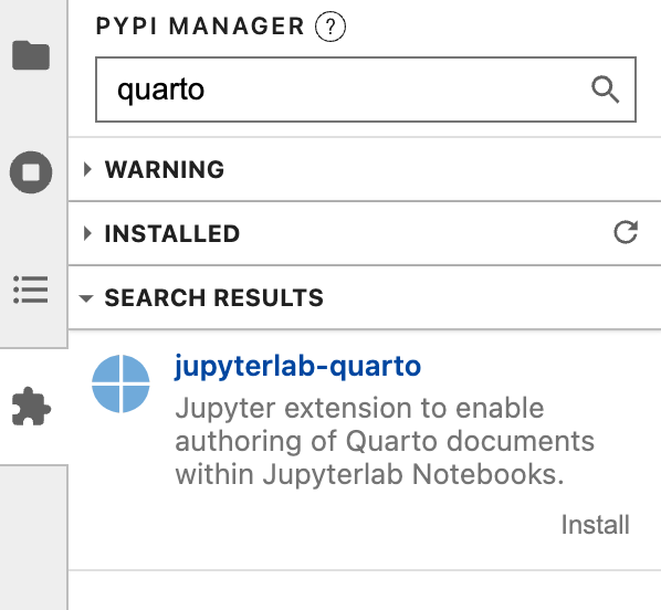

   

2. Using pip:

   Platform	Commands
   Mac/Linux	Terminal python3 -m pip install jupyterlab-quarto
   Windows	Terminal py -m pip install jupyterlab-quarto

JupyterLab 3

You can install the Quarto JupyterLab extension one of two ways:

1. Using pip, you can install the jupyterlab-quarto by executing:

   Platform	Commands
   Mac/Linux	Terminal python3 -m pip install jupyterlab-quarto==0.1.45
   Windows	Terminal py -m pip install jupyterlab-quarto==0.1.45

   This is the preferred way to install the JupyterLab Quarto extension as this takes advantage of traditional python packaging and doesn’t require a rebuild of JupyterLab to complete the installation.

2. In the JupyterLab UI, you can install the Quarto extension directly using the Extension Manager by searching for ‘Quarto’ and installing the @quarto/jupyterlab-quarto extension. To complete the installation you need to rebuild JupyterLab (you should see a prompt to complete this once you’ve installed the Quarto extension).

Clone the Template Repository

To follow this tutorial you’ll need your own copy of the template repository, including all of its branches.

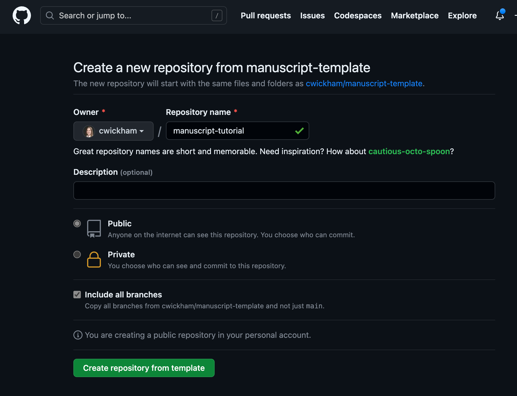
1. Head to GitHub to create a new repository from the template.

   Provide a Repository Name and make sure you check Include all branches. Then Create repository from template.

2. Once your repository is created, clone it to your local computer.

   You can do this any way you are comfortable, for instance in the Terminal, it might look like:

   Terminal

   git clone git@github.com:<username>/<repo-name>.git

   Where you use your own user name and repo name.

3. You’ll be working inside this directory throughout the tutorial, so if you are ready to proceed, navigate inside the directory, and start Jupyter Lab:

   Terminal

   cd manuscript-tutorial
   python3 -m jupyter lab

Template manuscript opened in Jupyter Lab

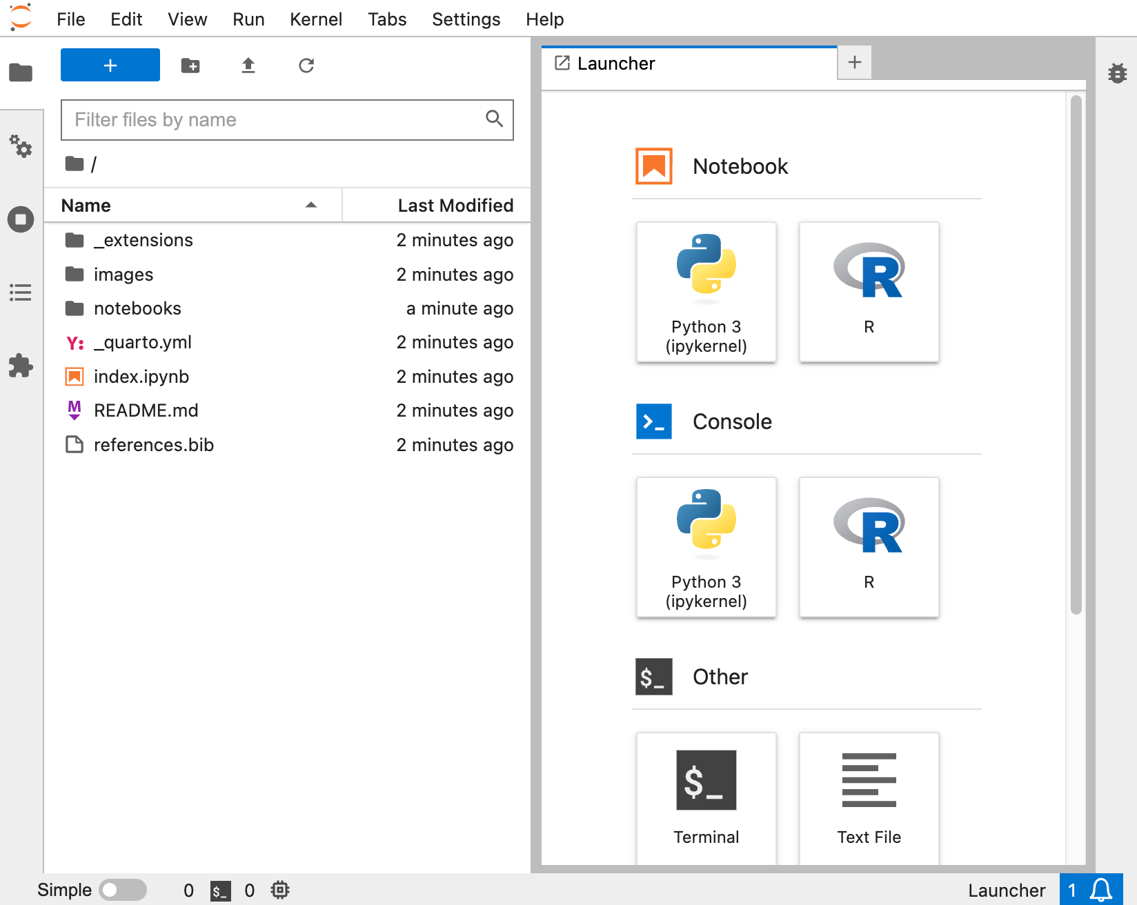
Project Files

At its simplest, a Quarto manuscript project has two files:

• A notebook file where you write your article: index.ipynb. This file contains:
  • document metadata, including article front matter (authors, affiliations, etc.) and Quarto options,
  • the article body, written using special Quarto markdown syntax that allows you to add things like cross references and citations, and
  • optionally, code, where you control if, or how, the code and its output appear in the article.
• A configuration file _quarto.yml that identifies the project as a Quarto manuscript and controls how your manuscript is put together.

This particular manuscript project includes some other files and folders, you’ll learn about these files as you work through this tutorial.

Workflow

The basic workflow for writing a manuscript in Quarto is to make changes to your article content in index.ipynb, preview the changes with Quarto, and repeat. Let’s try it out.

Open a new Terminal in Jupyter Lab and run:

Terminal

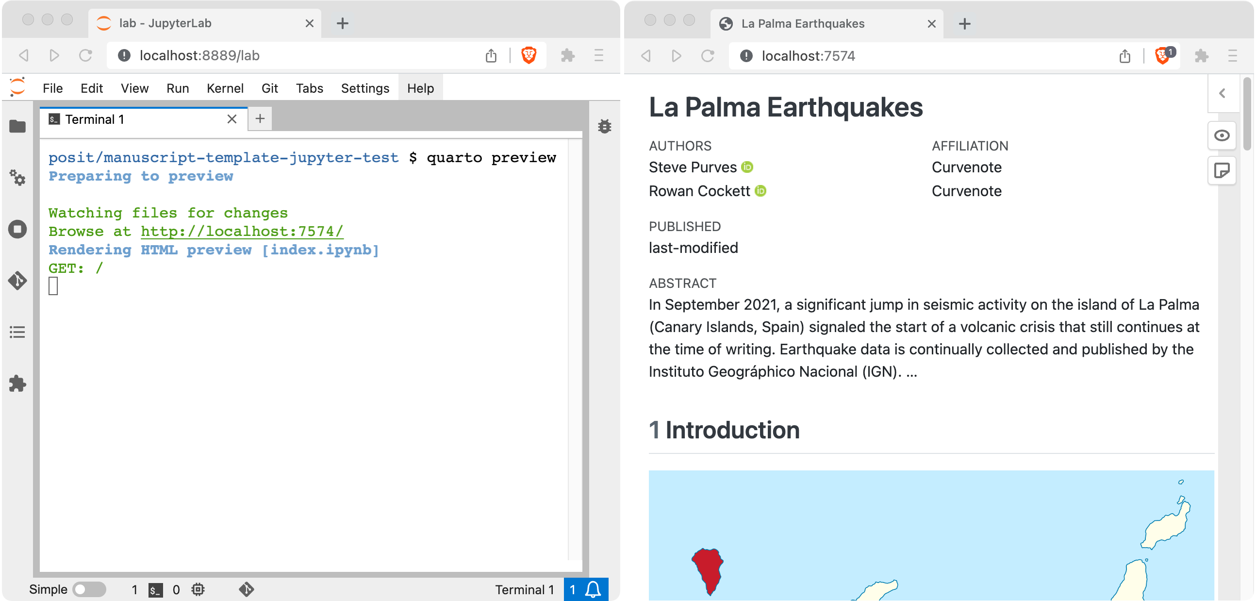
quarto preview

You’ll see some output from Quarto on the Terminal:

Terminal

$ quarto preview
Preparing to preview
[1/1] index.ipynb

Watching files for changes
Browse at http://localhost:3806/
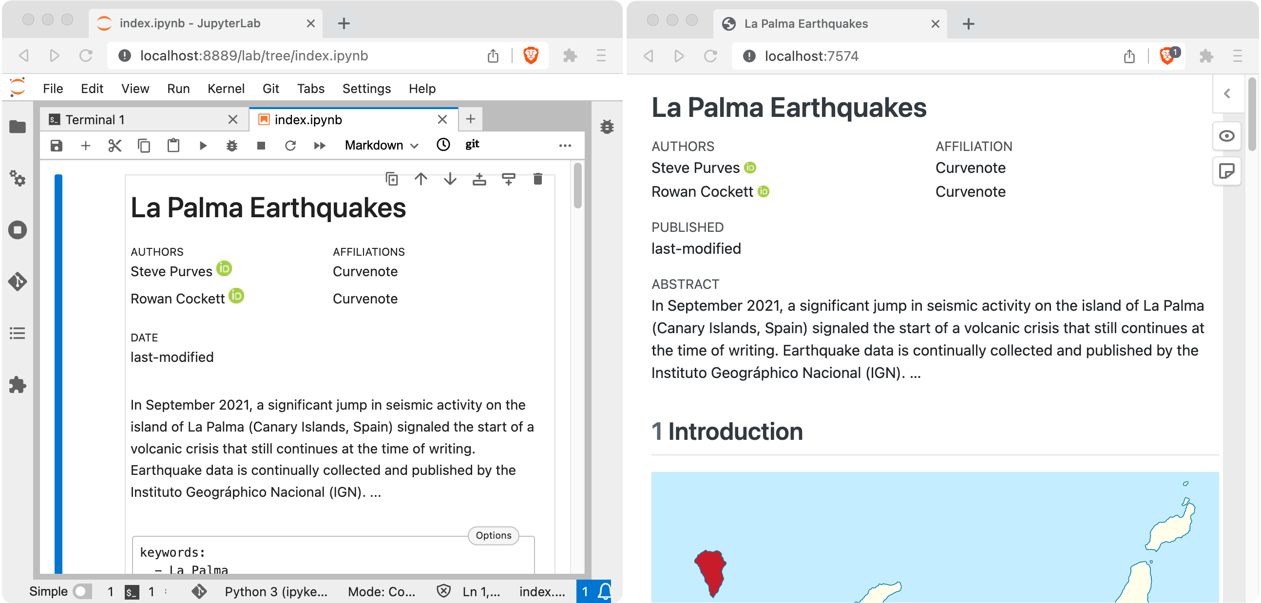
GET: /

And then, a browser window will open with a live preview of the manuscript.

You may find it helpful to move and resize your windows so that Jupyter Lab and the live preview are side by side.

The contents of the article is generated by index.ipynb. Go ahead and open this file in Jupyter Lab.

You’ll dive into the details of this file next, but for now let’s make a change and see what happens.

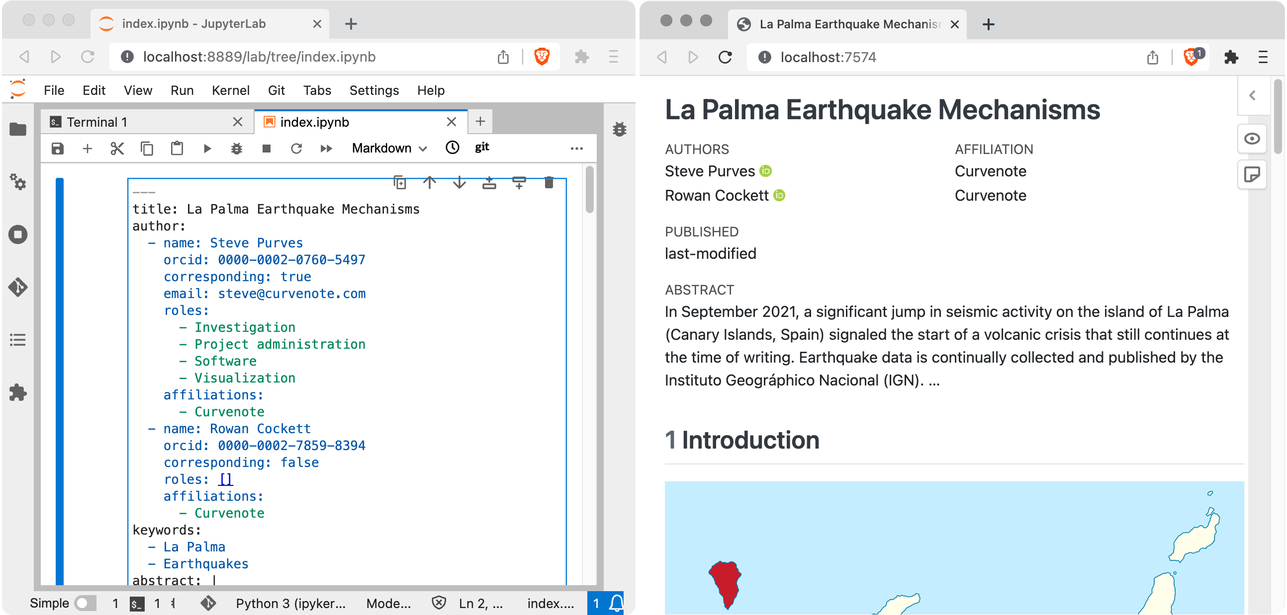
The first cell (starting with “La Palma Earthquakes”) is a Markdown cell, enter Edit mode in this cell, and find the line:

title: La Palma Earthquakes

Change the line to:

title: La Palma Earthquake Mechanisms

Save the notebook, and you’ll see the preview update automatically.

Tip

If you close the preview accidentally, you can navigate to it again by using the URL from the output in the Terminal, e.g. http://localhost:3806/. If you want to stop the preview, hit Crtl + C in the Terminal. You can start the preview again by running quarto preview.

Notebook Structure

The file index.ipynb is a Jupyter Notebook. Like any Jupyter Notebook it contains cells that could be raw, markdown or code. There are three features of this notebook that are Quarto specific:

• The first cell contains a YAML header that is used to set document metadata, including scholarly front matter. This cell must start and end with a line of three dashes (---), and within these lines, content is parsed as YAML. You’ll notice the cell itself is set to be a Markdown cell; this allows the Quarto Jupyter Lab Extension to visually emulate how some of these options will appear in the rendered document.

• The other markdown cells use Quarto specific markdown syntax to include things like figures, tables, equations, cross references and citations.

• Code cells may have special Quarto comments at the top that start with #|. These comments set Quarto options that control how the code and its output appear in the article.

The rest of this page walks you through the cells in this article from top to bottom, introducing you to the Quarto features you’ll most likely need to write a scholarly article.

Front Matter

The YAML header consists of key-value pairs set using the syntax key: value. The header is often extensive for articles because it is used to specify much of the scholarly front matter, like the authors and their affiliations, and the abstract.

Expand to see full YAML header for index.ipynb

title: La Palma Earthquakes
author:
  - name: Steve Purves
    orcid: 0000-0002-0760-5497
    corresponding: true
    email: steve@curvenote.com
    roles:
      - Investigation
      - Project administration
      - Software
      - Visualization
    affiliations:
      - Curvenote
  - name: Rowan Cockett
    orcid: 0000-0002-7859-8394
    corresponding: false
    roles: []
    affiliations:
      - Curvenote
keywords:
  - La Palma
  - Earthquakes
abstract: |
  In September 2021, a significant jump in seismic activity on the island of La Palma (Canary Islands, Spain) signaled the start of a volcanic crisis that still continues at the time of writing. Earthquake data is continually collected and published by the Instituto Geográphico Nacional (IGN). ...
plain-language-summary: |
  Earthquake data for the island of La Palma from the September 2021 eruption is found ...
key-points:
  - A web scraping script was developed to pull data from the Instituto Geogràphico Nacional into a machine-readable form for analysis
  - Earthquake events on La Palma are consistent with the presence of both mantle and crustal reservoirs.
date: last-modified
bibliography: references.bib
citation:
  container-title: Earth and Space Science
number-sections: true

For example, at the top level the header in index.ipynb sets the following keys: title, author, keywords, abstract, plain-language-summary, key-points, date, bibliography, citation, and number-sections.

You’ve seen how editing the title key updated the title of the article on the manuscript webpage. The title key is also used by the PDF and Word formats, but not all of the keys are used in all formats.

You can read more about setting the front matter for your article in Scholarly Front Matter.

Markdown

Markdown cells in the document will be processed by Quarto’s specific markdown syntax. Quarto’s markdown syntax is based on Pandoc Markdown, which in turn is based on John Gruber’s Markdown, the same markdown Jupyter Notebooks use.

As an example, the markdown to create the heading for the article’s introduction is:

## Introduction

First-level headings are reserved for the article title, so you’ll use second-level and deeper headings to structure the sections in your article.

If Markdown syntax is unfamiliar, you might want to read about Quarto Markdown Basics.

Computations

Python Examples

This section uses Python code examples, but Quarto also supports R, Julia and Observable.

You don’t need to rerun the Python code to follow along, but if you would like to, you’ll need the matplotlib and numpy packages.

Your article can include executable code. By default, code itself will not display in the article, but any output including tables and figures will. When you include code in your article, you’ll also get an additional link to the “Article Notebook” under Notebooks on the manuscript webpage. This is a rendered version of your article notebook that includes the code.

For example, index.ipynb, includes:

import matplotlib.pyplot as plt
import numpy as np
eruptions = [1492, 1585, 1646, 1677, 1712, 1949, 1971, 2021]

This code doesn’t appear in the rendered article, but does in the “Article Notebook”.

Rendered Article

Article Notebook

You can add Quarto options to code cells by adding a #| comment to the top, followed by the option in YAML syntax. For example, adding the echo option with the value true would look like this:

#| echo: true
import matplotlib.pyplot as plt
import numpy as np
eruptions = [1492, 1585, 1646, 1677, 1712, 1949, 1971, 2021]

The echo option describes whether the code is included in the rendered article. If you make this change and save index.ipynb, you’ll see this code now appears in the article.

You can find a list of all the code cell options available on the Jupyter Code Cell reference page.

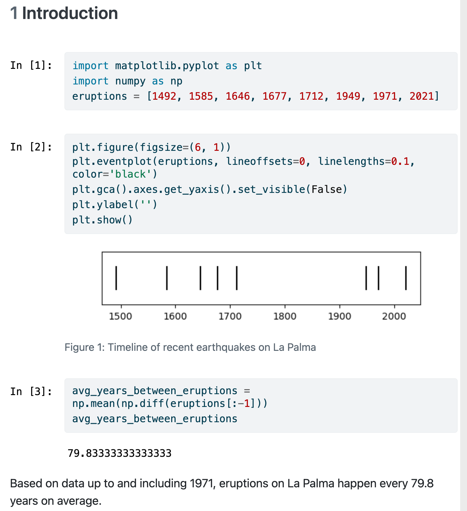
The next code cell creates a figure:

#| label: fig-timeline
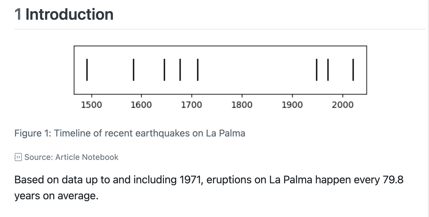
#| fig-cap: Timeline of recent earthquakes on La Palma
#| fig-alt: An event plot of the years of the last 8 eruptions on La Palma.

plt.figure(figsize=(6, 1))
plt.eventplot(eruptions, lineoffsets=0, linelengths=0.1, color='black')
plt.gca().axes.get_yaxis().set_visible(False)
plt.ylabel('')
plt.show()

The label option is used to add an identifier to code cell and its output, for example to allow cross referencing. The prefix fig- is required for figure cross references, but the suffix, in this case timeline, is up to you. You’ll learn more about Cross References below.

The option fig-cap provides the caption text displayed below the figure in the manuscript, and fig-alt provides alt text for the figure, helping your manuscript webpage to meet accessibility guidelines.

Computations are also a good way to include tables based on data. You can read more about doing this in the Quarto documentation on Tables from Computations.

If you have code output you don’t want to include in your article you can use output: false. For example, you may have a value that is helpful for writing your content, but you don’t want it to appear in the article itself. The next code cell is an example:

#| output: false
avg_years_between_eruptions = np.mean(np.diff(eruptions[:-1]))
avg_years_between_eruptions

If you are viewing the rendered “Article Notebook”, you’ll see the value of avg_years_between_eruptions displayed below this code, but the value does not appear in the rendered article.

If you’d like to exclude a cell and its output from both the article and the rendered notebook, you could use include: false instead:

#| include: false
avg_years_between_eruptions = np.mean(np.diff(eruptions[:-1]))
avg_years_between_eruptions

You can also use computed values directly in your article text by using inline code. Read more in Inline Code.

Rather than including computations directly in your article you can also embed outputs from other notebooks, read more below in Embedding Notebooks.

When is code executed?

By default, Quarto doesn’t execute any code in .ipynb notebooks. If you need to update cell outputs, run the appropriate cells, and save the notebook.

Citations

Article Citation

This section describes adding citations in the text of your article. The citation for your own article that is displayed at the bottom of the article webpage is controlled using Front Matter.

To add citations you need a bibliography file, .bib, containing the citation data. You can specify this file in the document YAML with the bibliography option. For example, the citation data for index.ipynb is stored in references.bib:

bibliography: references.bib

The file references.bib contains only one citation:

references.bib

@article{marrero2019,
  author = {Marrero, Jos{\' e} and Garc{\' i}a, Alicia and Berrocoso, Manuel and Llinares, {\' A}ngeles and Rodr{\' i}guez-Losada, Antonio and Ortiz, R.},
  journal = {Journal of Applied Volcanology},
  year = {2019},
  month = {7},
  pages = {},
  title = {Strategies for the development of volcanic hazard maps in monogenetic volcanic fields: the example of {La} {Palma} ({Canary} {Islands})},
  volume = {8},
  doi = {10.1186/s13617-019-0085-5},
}

To cite an article from the bibliography in your text, you use @ followed by the citation identifier, e.g. marrero2019. For example, the article includes this line citing this reference:

Studies of the magma systems feeding the volcano, such as @marrero2019, have proposed ...

This renders as:

Studies of the magma systems feeding the volcano, such as Marrero et al. (2019), have proposed …

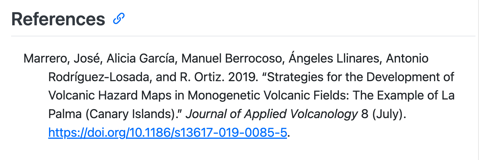
Hovering over the citation text reveals the full reference details. Clicking on the citation takes a reader to the reference in the References section at the end of the article:

The above citation is an example where the author’s names are incorporated into the sentence itself. Another common style is to place the citation within parentheses, often at the end of a sentence. You can achieve this by enclosing the citation syntax in square brackets [. For example,

A prior study of the magma systems feeding the volcano proposed that there are two main magma reservoirs feeding the Cumbre Vieja volcano [@marrero2019].

This renders as:

A prior study of the magma systems feeding the volcano proposed that there are two main magma reservoirs feeding the Cumbre Vieja volcano (Marrero et al. 2019).

There are many other syntax variations to include page numbers, chapters, or exclude the author names. You can read more in the Citations documentation.

Cross References

Quarto can generate cross references that keep track of numbering and linking for you. The general syntax for a cross reference is an @ followed by a label. For example, to reference the timeline figure, you could write:

@fig-timeline

When rendered, cross references include a word to indicate the type of object being referenced, like “Figure” or “Table”. So for instance, this line in index.ipynb:

Eight eruptions have been recorded since the late 1400s (@fig-timeline).

Results in the text:

Eight eruptions have been recorded since the late 1400s (Figure 1).

Where “Figure 1” is also a link to the appropriate figure.

The labels you add to elements must have the appropriate prefix to allow cross referencing:

Element	Label Prefix	Rendered Cross Reference
Figure	fig-	Figure 1
Table	tbl-	Table 1
Equation	eq-	Equation 1
Section	sec-	Section 1

You’ve already seen you can add a label to output generated by code using the label code chunk option. You’ll see how to add labels to non-code generated elements, like equations, tables, and static figures, as you learn about them below.

To cross reference sections your document YAML header must also include:

number-sections: true

You can add a label to a section heading in curly braces after the heading, e.g:

## Data & Methods {#sec-data-methods}

You can then reference this section in the text, like:

Data and methods are discussed in @sec-data-methods.

Which will be rendered as:

Data and methods are discussed in Section 2.

You can read more about the types of objects that can be referenced, including code listings, and mathematical theorems, as well as some of the options to control how references appear in the Quarto Cross References documentation.

Equations

Quarto markdown can include equations specified in LaTeX notation. Use single dollar signs ($) to add an equation inline or double dollar signs ($$) to add a display equation. Both of these are illustrated in the following paragraph in index.ipynb:

Let $x$ denote the number of eruptions in a year. Then, $x$ can be modeled by a Poisson distribution

$$
p(x) = \frac{e^{-\lambda} \lambda^{x}}{x !}
$$ {#eq-poisson}

where $\lambda$ is the rate of eruptions per year. Using @eq-poisson, the probability of an eruption in the next $t$ years can be calculated.

Notice the display equation has a label added in curly braces after the closing $$. This allows it to be referenced using @eq-poisson in the text.

When rendered, this displays as:

Let \(x\) denote the number of eruptions in a year. Then, \(x\) can be modeled by a Poisson distribution \[ p(x) = \frac{e^{-\lambda} \lambda^{x}}{x !} \tag{1}\] where \(\lambda\) is the rate of eruptions per year. Using Equation 1, the probability of an eruption in the next \(t\) years can be calculated.

Tables

Tables can be added inline with what is known as pipe syntax. As an example, in index.ipynb a table of earthquakes is specified as:

| Name                 | Year   |
| -------------------- | ------ |
| Current              | 2021   |
| Teneguía             | 1971   |
| Nambroque            | 1949   |
| El Charco            | 1712   |
| Volcán San Antonio   | 1677   |
| Volcán San Martin    | 1646   |
| Tajuya near El Paso  | 1585   |
| Montaña Quemada      | 1492   |

: Recent historic eruptions on La Palma {#tbl-history}

Columns are separated by pipes (|), and the dashes (-) in the second row separate the header row from the rest of the table. A caption can be provided with a line starting with :. A label that can be used for cross references is added at the end of the caption inside curly braces. Like figures, the label prefix tbl- is required for cross references, but the suffix is up to you.

You can learn more about tables in Quarto, including an alternative syntax known as grid tables, on the Tables page in the Quarto documentation.

Static Figures

To include a figure from a file, the markdown syntax looks like:

![Caption](file_path_to_image)

For example, to include the la-palma-map.png image from the images/ folder in the project, along with the caption “Map of La Palma”, you would write:

![Map of La Palma](images/la-palma-map.png)

Image File Location

You don’t have to store your images in a folder called images/, although it is a common convention. Your images can be anywhere inside your manuscript project directory, just make sure you include the full path to the image, relative to the location of index.ipynb.

The actual markdown in index.ipynb includes a further attribute, #fig-map inside curly braces following the image path to provide a label for cross references:

![Map of La Palma](images/la-palma-map.png){#fig-map}

Another attribute that you may wish to add is fig-alt, the alt text to be provided for the image. For example:

![Map of La Palma](images/la-palma-map.png){#fig-map fig-alt="A map of the Canary Islands. The second most west island, La Palma, is highlighted."}

You can read more about including figures in Quarto documents, including how to resize figures and arrange multiple figures, on the Quarto docs Figures page.

External Embeds

An alternative to including computations directly in the article notebook, is to embed output from other notebooks. This manuscript project includes the notebook data-screening.ipynb in the notebooks/ folder.

To embed output from a notebook, you can use the embed shortcode. Quarto shortcodes are special markdown directives that generate content. The embed shortcode is used in main article file in the line:

index.ipynb

{{< embed notebooks/data-screening.ipynb#fig-spatial-plot >}}

The double curly braces ({{) and angle brackets (<) indicate this is a shortcode. The embed shortcode requires a path to a notebook cell. In this case, it’s the file path to data-screening.ipynb, followed by # and a cell identifier. Here, the cell identifier is the cell label, set using the Quarto cell option label in code cell in the data-screening.ipynb notebook:

data-screening.ipynb

#| label: fig-spatial-plot
#| fig-cap: "Locations of earthquakes on La Palma since 2017."
#| fig-alt: "A scatterplot of earthquake locations plotting latitude 
#|   against longitude."
from matplotlib import colormaps
cmap = colormaps['viridis_r']
ax = df.plot.scatter(x="Longitude", y="Latitude", 
                     s=40-df["Depth(km)"], c=df["Magnitude"], 
                     figsize=(12,10), grid="on", cmap=cmap)
colorbar = ax.collections[0].colorbar
colorbar.set_label("Magnitude")

plt.show()

Just like any figure, using a label starting with fig- allows it to be cross referenced in the text. Any other options, like the figure caption (fig-cap) and alt text (fig-alt), can also be set in the source notebook.

In this manuscript, the notebook data-screening.ipynb isn’t reproducible: you can’t regenerate all the outputs because some inputs (e.g. the data) aren’t included in the project. However, you can change the Quarto cell options without rerunning the code cells in the notebook. If you edit the caption to:

#| fig-cap: "Earthquakes on La Palma since 2017."

When you save data-screening.ipynb, you’ll find the preview updates and the caption is reflected in the article itself.

Up Next

You’ve now covered the main features of Quarto for authoring a manuscript. You’ve edited index.ipynb, added resources like figures, notebooks or bibliographic data, and previewed the result.

Once, you are happy with the changes you’ve made, you’ll need update your public manuscript webpage.

Head on to Publishing to learn how to publish and share your manuscript with the world.