Code
library(ggplot2)
dat <- data.frame(cond = rep(c("A", "B"), each=10),
xvar = 1:20 + rnorm(20,sd=3),
yvar = 1:20 + rnorm(20,sd=3))
ggplot(dat, aes(x=xvar, y=yvar)) +
geom_point(shape=1) +
geom_smooth() 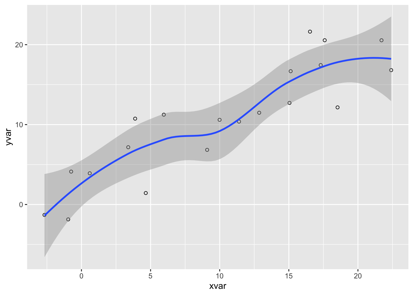
There are wide variety of options available to customize the display of source code within HTML documents, including:
Details on using all of these options are provided below.
For many documents you may want to hide all of the executable source code used to produce dynamic outputs. You can do this by specifying echo: false in the document execute options. For example:
---
title: "My Document"
execute:
  echo: false
jupyter: python3
---
Note that we can override this option on a per code-block basis. For example:
```{python}
#| echo: true

import matplotlib.pyplot as plt
plt.plot([1,2,3,4])
plt.show()
```
Code block options are included in a special comment at the top of the block (lines at the top prefaced with #| are considered options).
Use the code-fold option to include code but have it hidden by default using the HTML <details> tag. For example, click the Code button to see the code that produced this plot.
library(ggplot2)
dat <- data.frame(cond = rep(c("A", "B"), each=10),
                  xvar = 1:20 + rnorm(20,sd=3),
                  yvar = 1:20 + rnorm(20,sd=3))

ggplot(dat, aes(x=xvar, y=yvar)) +
  geom_point(shape=1) +
  geom_smooth()
Here we specify both code-fold: true as well as custom summary text (the default is just “Code” as shown above):
format:
  html:
    code-fold: true
    code-summary: "Show the code"
Valid values for code-fold include:
| Value | Behavior |
|---|---|
false |
No folding (default) |
true |
Fold code (initially hidden) |
show |
Fold code (initially shown) |
Use the code-fold and code-summary chunk attributes to control this on a chunk-by-chunk basis:
```{r}
#| code-fold: true
#| code-summary: "Show the code"
```In some cases the width of source code will overflow the available horizontal display space. By default, this will result in a horizontal scroll bar for the code block. However if you prefer not to have scrollbars you can have the longer lines wrap instead.
To set the global default behavior use the code-overflow option. For example:
format:
  html:
    code-overflow: wrap
Valid values for code-overflow are:
| Option | Description |
|---|---|
scroll |
Scroll code blocks that exceed available width (default, corresponds to white-space: pre). |
wrap |
Wrap lines of code that exceed available width (corresponds to white-space: pre-wrap). |
You can also override the global default on a per-code-block basis. For computational cells you do this with the code-overflow cell option:
```{python}
#| code-overflow: wrap

# very long line of code....
```
For a static code block, add the .code-overflow-scroll or .code-overflow-wrap CSS class:
```{.python .code-overflow-wrap}
# very long line of code....
```
Note that irrespective of these options, code will always wrap within printed HTML output (as it would otherwise be clipped off the edge of the page).
You can include a Code menu in the header of your document that provides various tools for readers to interact with the source code. Specify code-tools: true to activate these tools:
format:
  html:
    code-fold: true
    code-tools: true
If you have a document that includes folded code blocks then the Code menu will present options to show and hide the folded code as well as view the full source code of the document:
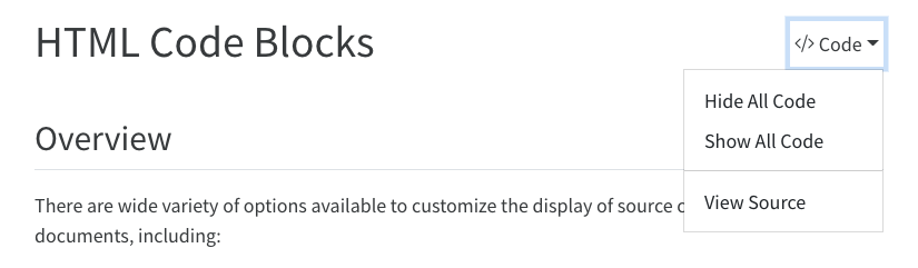
This document specifies code-tools: true in its options so you should see the Code menu above next to the main header.
You can control which of these options are made available as well as the “Code” caption text using sub-options of code-tools. For example, here we specify that we want only “View Source” (no toggling of code visibility) and no caption on the code menu:
format:
  html:
    code-tools:
      source: true
      toggle: false
      caption: none
By default, the source code is embedded in the document and shown in a popup window like this:
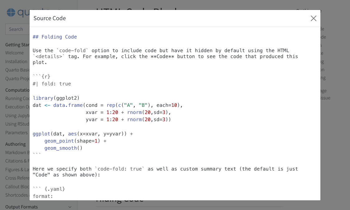
You can alternatively specify a URL for the value of source:
format:
  html:
    code-tools:
      source: https://github.com/quarto-dev/quarto-web/blob/main/index.md
If you are within a project and have specified a repo-url option then you can just use repo and the correct link to your source file will be generated:
format:
  html:
    code-tools:
      source: repo
Note that the code-tools option is not available when you disable the standard HTML theme (e.g. if you specify the theme: none option).
By default code blocks are rendered with a left border whose color is derived from the current theme. You can customize code chunk appearance with some simple options that control the background color and left border. Options can either be booleans to enable or disable the treatment or can be legal CSS color strings (or they could even be SASS variable names!).
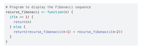
Here is the default appearance for code blocks (code-block-bg: true):
You can instead use a left border treatment using the code-block-border-left option:
code-block-border-left: true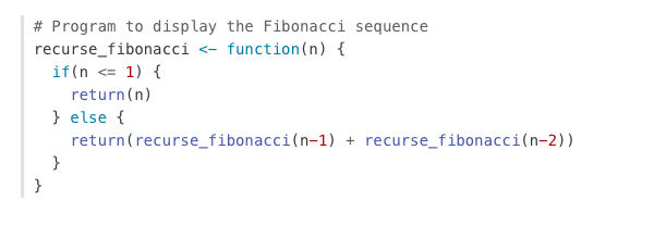
You can combine a background and border treatment as well as customize the left border color:
code-block-bg: true
code-block-border-left: "#31BAE9"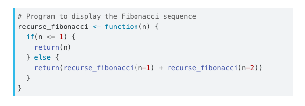
Use the filename attribute on code blocks If you are documenting the contents of a file and want to be especially clear about the name of the file the code is associated with.
For example, the following code:
```{.python filename="matplotlib.py"}
import matplotlib.pyplot as plt
plt.plot([1,23,2,4])
plt.show()
```
Results in this HTML output:
matplotlib.py
import matplotlib.pyplot as plt
plt.plot([1,23,2,4])
plt.show()
Non-HTML formats will still have the filename, but it will simply be shown in bold above the code block.
Pandoc will automatically highlight syntax in fenced code blocks that are marked with a language name. For example:
```python
1 + 1
```
Pandoc can provide syntax highlighting for over 140 different languages (see the output of quarto pandoc --list-highlight-languages for a list of all of them). If you want to provide the appearance of a highlighted code block for a language not supported, just use default as the language name.
You can specify the code highlighting style using syntax-highlighting and specifying one of the supported themes. These themes are “adaptive”, which means they will automatically switch between a dark and light mode based upon the theme of the website. These are designed to work well with sites that include a dark and light mode.
All of the standard Pandoc themes are also available:
As well as an additional set of extended themes, including:
The syntax-highlighting option determines which theme is used. For example:
syntax-highlighting: githubHighlighting themes can provide either a single highlighting definition or two definitions, one optimized for a light colored background and another optimized for a dark color background. When available, Quarto will automatically select the appropriate style based upon the code chunk background color’s darkness. Users may always opt to specify the full name (e.g. atom-one-dark) to by pass this automatic behavior.
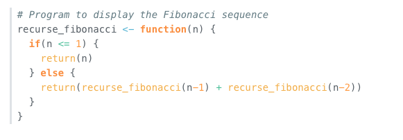
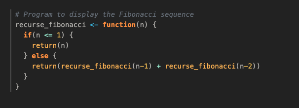
By default, code is highlighted using the arrow theme, which is optimized for accessibility. We’ve additionally introduced the arrow-dark theme which is designed to provide accessible highlighting against dark backgrounds.
Examples of the light and dark themes:
![]()
![]()
In addition to the built in themes available for syntax highlighting, you can also specify your own syntax highlighting by providing the path to a valid theme file (which is based upon the KDE XML syntax highlighting descriptions). Highlighting is implemented using skylighting.
For example:
---
syntax-highlighting: custom.theme
---
In addition, if you’d like to provide adaptive themes, you may also pass both a light and dark theme file:
---
syntax-highlighting:
  light: custom-light.theme
  dark: custom-dark.theme
---
Note that as with adaptive text higlighting themes, when you provide a dark and light syntax-highlighting, background colors specified in the themes will be ignored in favor of the overall theme specified background colors.
You can add annotations to lines of code in code blocks and executable code cells. See Code Annotation for full details.
If you want to display line numbers alongside the code block, add the code-line-numbers option. For example:
format:
  html:
    code-line-numbers: true
Here’s how a code block with line numbers would display:
You can also enable line numbers for an individual code block using the code-line-numbers attribute. For example:
``` {.python code-line-numbers="true"}
import matplotlib.pyplot as plt
plt.plot([1,23,2,4])
plt.show()
```The documentation on computations covers how to include executable code blocks (code which is actually executed, with its output being included in the rendered document). We won’t additionally cover that here, but we will talk about how to include code blocks that demonstrate executable syntax (e.g. for writing a tutorial).
Often you’ll want to include a fenced code block purely as documentation (not executable). You can do this by using two curly braces around the language (e.g. python, r, etc.) rather than one. For example:
```{{python}}
1 + 1
```
Will be output into the document as:
```{python}
1 + 1
```
If you want to show an example with multiple code blocks and other markdown, just enclose the entire example in 4 backticks (e.g. ````) and use the two curly brace syntax for code blocks within. For example:
````
---
title: "My document"
---

Some markdown content.

```{{python}}
1 + 1
```

Some additional markdown content.

````The code-link option enables hyper-linking of functions within code blocks to their online documentation:
format:
  html:
    code-link: true
Code linking is currently implemented only for the knitr engine (via the downlit package). A limitation of downlit currently prevents code linking if code-line-numbers and/or code-annotations are also true.