```{python}
1 + 1
```2There are a wide variety of options available for customizing output from executed code. All of these options can be specified either globally (in the document front-matter) or per code-block. For example, here’s a modification of the Python example to specify that we don’t want to “echo” the code into the output document:
---
title: "My Document"
execute:
  echo: false
jupyter: python3
---
Note that we can override this option on a per code-block basis. For example:
```{python}
#| echo: true

import matplotlib.pyplot as plt
plt.plot([1,2,3,4])
plt.show()
```
Code block options are included in a special comment at the top of the block (lines at the top prefaced with #| are considered options).
Options available for customizing output include:
| Option | Description |
|---|---|
eval |
Evaluate the code chunk (if false, just echos the code into the output). |
echo |
Include the source code in output |
output |
Include the results of executing the code in the output (true, false, or asis to indicate that the output is raw markdown and should not have any of Quarto’s standard enclosing markdown). |
warning |
Include warnings in the output. |
error |
Include errors in the output (note that this implies that errors executing code will not halt processing of the document). |
include |
Catch all for preventing any output (code or results) from being included (e.g. include: false suppresses all output from the code block). |
renderings |
Specify rendering names for the plot or table outputs of the cell, e.g. [light, dark] |
Here’s a Knitr example with some of these additional options included:
---
title: "Knitr Document"
execute:
echo: false
---
```{r}
#| warning: false
library(ggplot2)
ggplot(airquality, aes(Temp, Ozone)) +
geom_point() +
geom_smooth(method = "loess", se = FALSE)
```
```{r}
summary(airquality)
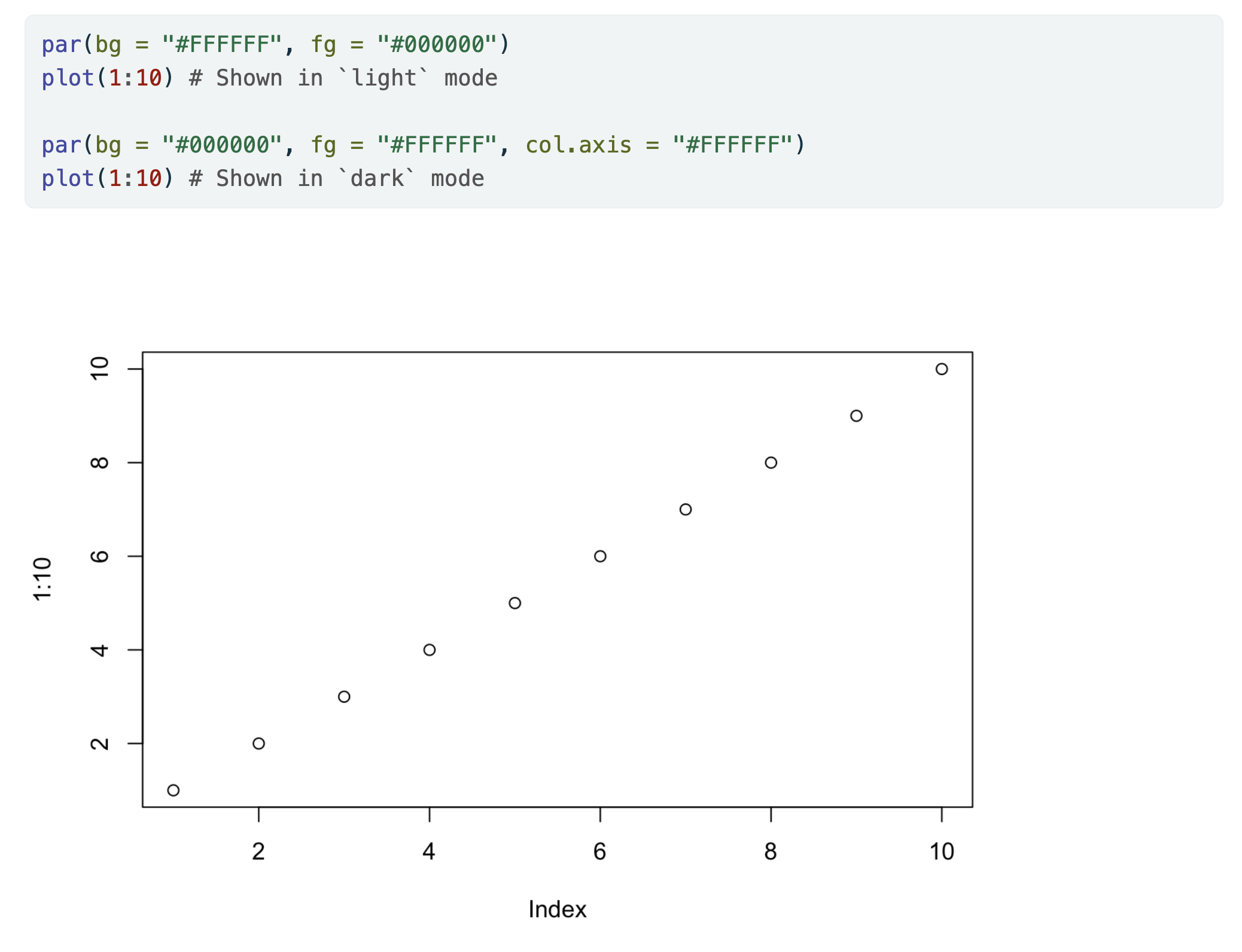
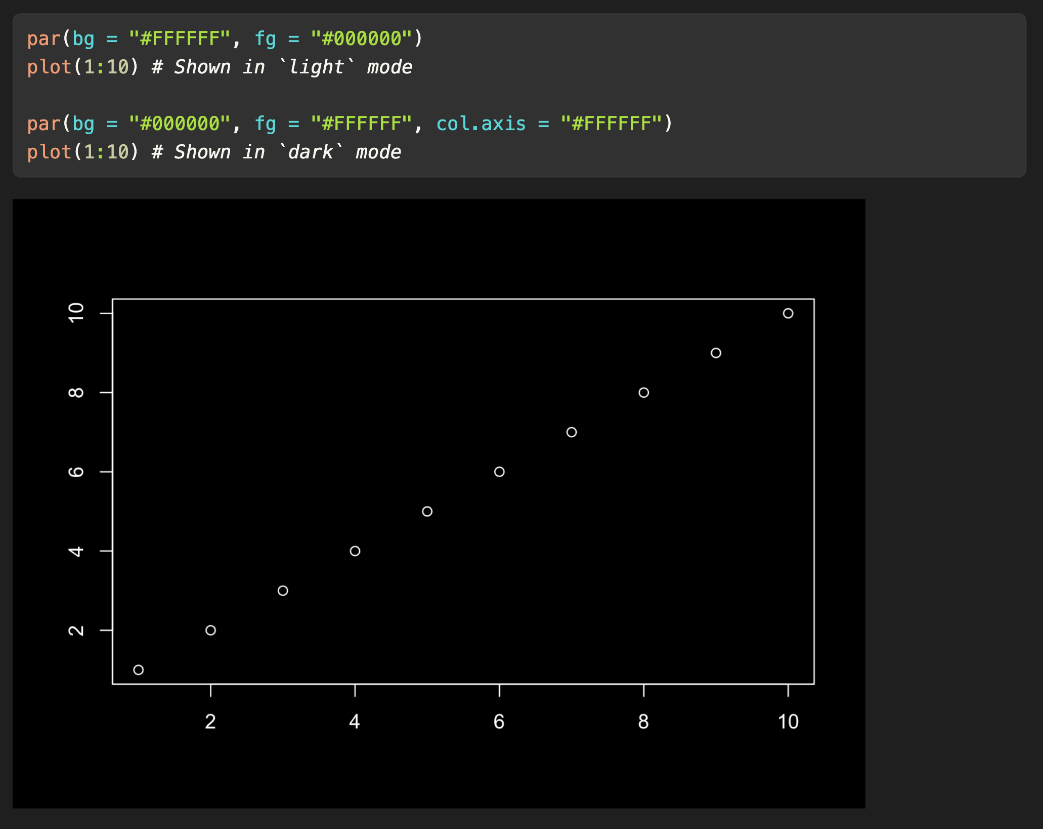
```Here is an example of using renderings to provide light and dark versions of a plot. Note that the number of cell outputs must match the number of renderings.
---
title: "Dark mode"
format:
  html:
    theme:
      light: flatly
      dark: darkly
---

```{r}
#| renderings: [light, dark]
par(bg = "#FFFFFF", fg = "#000000")
plot(1:10) # Shown in `light` mode

par(bg = "#000000", fg = "#FFFFFF", col.axis = "#FFFFFF")
plot(1:10) # Shown in `dark` mode
```
The renderings cell option does not currently work correctly with cell cross-reference options (label starting with fig-, tbl-, etc.) or cell caption options (fig-cap, tbl-cap, etc.).
To combine renderings with crossrefs and/or captions, use the fenced div syntax:
---
title: "Dark mode"
format:
  html:
    theme:
      light: flatly
      dark: darkly
---

::: {#fig-caption-crossref}

```{r}
#| label: caption-crossref
#| renderings: [light, dark]
par(bg = "#FFFFFF", fg = "#000000")
plot(1:10) # Shown in `light` mode


par(bg = "#000000", fg = "#FFFFFF", col.axis = "#FFFFFF")
plot(1:10) # Shown in `dark` mode
```

Light and dark renderings with a caption and crossref

:::
Note the use of a label that is not a cross-reference, i.e. that does not start with one of the cross reference types. It is a good practice to have named cells with label, for debuggability and stable resource names. However, cross-reference labels that start with fig-, tbl-, etc., will not work with renderings.
When using the Knitr engine, you can also use any of the available native options (e.g. collapse, tidy, comment, etc.). See the Knitr options documentation for additional details. You can include these native options in option comment blocks as shown above, or on the same line as the {r} as shown in the Knitr documentation.
The Knitr engine can also conditionally evaluate a code chunk using objects or expressions. See Using R: Knitr Options.
There are a number of ways to control the default width and height of figures generated from code. First, it’s important to know that Quarto sets a default width and height for figures appropriate to the target output format. Here are the defaults (expressed in inches):
| Format | Default |
|---|---|
| Default | 7 x 5 |
| HTML Slides | 9.5 x 6.5 |
| HTML Slides (reveal.js) | 9 x 5 |
| 5.5 x 3.5 | |
| PDF Slides (Beamer) | 10 x 7 |
| PowerPoint | 7.5 x 5.5 |
| MS Word, ODT, RTF | 5 x 4 |
| EPUB | 5 x 4 |
| Hugo | 8 x 5 |
These defaults were chosen to provide attractive well proportioned figures, but feel free to experiment to see whether you prefer another default size. You can change the default sizes using the fig-width and fig-height options. For example:
---
title: "My Document"
format:
  html:
    fig-width: 8
    fig-height: 6
  pdf:
    fig-width: 7
    fig-height: 5
---
How do these sizes make their way into the engine-level defaults for generating figures? This differs by engine:
For the Knitr engine, these values become the default values for the fig.width and fig.height chunk options. You can override these default values via chunk level options.
For Python, these values are used to set the Matplotlib figure.figsize rcParam (you can of course manually override these defaults for any given plot).
For Julia, these values are used to initialize the default figure size for the Plots.jl GR backend.
If you are using another graphics library with Jupyter and want to utilize these values, you can read them from QUARTO_FIG_WIDTH and QUARTO_FIG_HEIGHT environment variables.
When using the Jupyter engine, fig-width and fig-height are only supported if specified at the document- or project-level. However, when using the Knitr engine, these options are also supported as code cell options on a per-cell basis.
You can specify the caption and alt text for figures generated from code using the fig-cap and fig-alt options. For example, here we add these options to a Python code cell that creates a plot:
```{python}
#| fig-cap: "Polar axis plot"
#| fig-alt: "A line plot on a polar axis"

import numpy as np
import matplotlib.pyplot as plt

r = np.arange(0, 2, 0.01)
theta = 2 * np.pi * r
fig, ax = plt.subplots(subplot_kw={'projection': 'polar'})
ax.plot(theta, r)
ax.set_rticks([0.5, 1, 1.5, 2])
ax.grid(True)
plt.show()
```Jupyter, Knitr and OJS all support executing inline code within markdown (e.g. to allow narrative to automatically use the most up to date computations). See Inline Code for details.
The output: asis option enables you to generate raw markdown output. When output: asis is specified none of Quarto’s standard enclosing divs will be included. For example, here we specify output: asis in order to generate a pair of headings:
```{python}
#| echo: false
#| output: asis

print("# Heading 1\n")
print("## Heading 2\n")
```
```{r}
#| echo: false
#| output: asis
cat("# Heading 1\n")
cat("## Heading 2\n")
```Which generates the following output:
# Heading 1

## Heading 2
Note that we also include the echo: false option to ensure that the code used to generate markdown isn’t included in the final output.
If we had not specified output: asis the output, as seen in the intermediate markdown, would have included Quarto’s .cell-output div:
::: {.cell-output-stdout}
```
# Heading 1

## Heading 2

```
:::
For the Jupyter engine, you can also create raw markdown output using the functions in IPython.display. For example:
```{python}
#| echo: false
radius = 10
from IPython.display import Markdown
Markdown(f"The _radius_ of the circle is **{radius}**.")
```If you are using the Knitr cell execution engine, you can specify default document-level Knitr chunk options in YAML. For example:
---
title: "My Document"
format: html
knitr:
  opts_chunk:
    collapse: true
    comment: "#>"
    R.options:
      knitr.graphics.auto_pdf: true
---
You can additionally specify global Knitr options using opts_knit.
The R.options chunk option is a convenient way to define R options that are set temporarily via options() before the code chunk execution, and immediately restored afterwards.
In the example above, we establish default Knitr chunk options for a single document. You can also add shared knitr options to a project-wide _quarto.yml file or a project-directory scoped _metadata.yml file.
When multiple expressions are present in a code cell, by default, only the last top-level expression is captured in the rendered output. For example, consider the code cell:
```{python}
"first"
"last"
```
When rendered to HTML the output generated is:
'last'This behavior corresponds to the last_expr setting for Jupyter shell interactivity.
You can control this behavior with the ipynb-shell-interactivity option. For example, to capture all top-level expressions set it to all:
---
title: All expressions
format: html
ipynb-shell-interactivity: all
---
Now the above code cell results in the output:
'first'

'last'For dashboards the default setting of ipynb-shell-interactivity is all.
On the way from markdown input to final output, there are some intermediate files that are created and automatically deleted at the end of rendering. You can use the following options to keep these intermediate files:
| Option | Description |
|---|---|
keep-md |
Keep the markdown file generated by executing code. |
keep-ipynb |
Keep the notebook file generated from executing code (applicable only to markdown input files) |
For example, here we specify that we want to keep the jupyter intermediate file after rendering:
---
title: "My Document"
execute:
  keep-ipynb: true
jupyter: python3
---If you are writing a tutorial or documentation on using Quarto code blocks, you’ll likely want to include the fenced code delimiter (e.g. ```{python}) in your code output to emphasize that executable code requires that delimiter. You can do this using the echo: fenced option. For example, the following code block:
```{python}
#| echo: fenced
1 + 1
```
Will be rendered as:
```{python}
1 + 1
```2This is especially useful when you want to demonstrate the use of cell options. For example, here we demonstrate the use of the output and code-overflow options:
```{python}
#| echo: fenced
#| output: false
#| code-overflow: wrap
1 + 1
```
This code block appears in the rendered document as:
```{python}
#| output: false
#| code-overflow: wrap
1 + 1
```
Note that all YAML options will be included in the fenced code output except for echo: fenced (as that might be confusing to readers).
This behavior can also be specified at the document level if you want all of your executable code blocks to include the fenced delimiter and YAML options:
---
title: "My Document"
format: html
execute:
  echo: fenced
---Often you’ll want to include a fenced code block purely as documentation (not executable). You can do this by using two curly braces around the language (e.g. python, r, etc.) rather than one. For example:
```{{python}}
1 + 1
```
Will be output into the document as:
```{python}
1 + 1
```
If you want to show an example with multiple code blocks and other markdown, just enclose the entire example in 4 backticks (e.g. ````) and use the two curly brace syntax for code blocks within. For example:
````
---
title: "My document"
---

Some markdown content.

```{{python}}
1 + 1
```

Some additional markdown content.

````Earlier we said that the engine used for computations was determined automatically. You may want to customize this—for example you may want to use the Jupyter R kernel rather than Knitr, or you may want to use Knitr with Python code (via reticulate).
Here are the basic rules for automatic binding:
| Extension | Engine Binding |
|---|---|
| .qmd | Use Knitr engine if an Use Jupyter engine if any other executable code block (e.g. Use no engine if no executable code blocks are discovered. |
| .ipynb | Jupyter engine |
| .Rmd | Knitr engine |
| .md | No engine (note that if an md document does contain executable code blocks then an error will occur) |
If your quarto document includes both {python} and {r} code blocks, then quarto will automatically use Knitr engine and reticulate R package to execute the python content.
For .qmd files in particular, you can override the engine used via the engine option. For example:
engine: jupyterengine: knitrYou can also specify that no execution engine should be used via engine: markdown.
The presence of the knitr or jupyter option will also override the default engine:
knitr: truejupyter: python3Variations with additional engine-specific options also work to override the default engine:
knitr:
  opts_knit:
    verbose: true
jupyter:
kernelspec:
display_name: Python 3
language: python
name: python3Using shell commands (from Bash, Zsh, etc.) within Quarto computational documents differs by engine. If you are using the Jupyter engine you can use Jupyter shell magics. For example:
---
title: "Using Bash"
engine: jupyter
---

```{python}
!echo "foo"
```
Note that ! preceding echo is what enables a Python cell to be able to execute a shell command.
If you are using the Knitr engine you can use ```{bash} cells, for example:
---
title: "Using Bash"
engine: knitr
---

```{bash}
echo "foo"
```
Note that the Knitr engine also supports ```{python} cells, enabling the combination of R, Python, and Bash in the same document
In some cases you want code execution itself — not just visibility of its output — to depend on the active output format. For example, when rendering to PDF you may want to skip a cell that loads an interactive HTML widget, rather than execute it and hide the result.
Quarto exposes the current rendering context in the QUARTO_EXECUTE_INFO environment variable. Cells can read this variable to detect the active format and branch accordingly. See Execution Context Information for the full JSON schema and examples in R, Python, and Julia.
This complements format-based conditional content, which controls visibility of already-executed output. QUARTO_EXECUTE_INFO lets you skip work, choose a different code path, or load a different library before any output is produced.