Libraries

Overview

There are three types of library you’ll generally use with OJS:

1. Observable core libraries automatically available in every document.

2. Third-party JavaScript libraries from npm and ObservableHQ.

3. Custom libraries you and/or your colleagues have created

In this document we’ll provide a high-level overview of the core libraries and some examples of using third-party libraries (D3 and Arquero). Creating your own libraries is covered in the article on Code Reuse.

Stdlib

The Observable standard library provides the core capabilities that underlie rendering content and loading code and data. Some particularly important components of the standard library include:

Component	Description
DOM	Dynamically creating DOM elements
FileAttachments	Reading files in a variety of formats
require	Importing third-party modules from NPM and GitHub

You can find complete documentation for the standard library at https://github.com/observablehq/stdlib.

Note

Quarto always embeds a specific version of ObservableHQ’s runtime, which means that Quarto might be behind the very latest ObservableHQ version on their website. If you need to use the latest version of Plot (or other core libraries), you can use the import function to import the latest version directly from a CDN. For example:

Plot = import("https://cdn.jsdelivr.net/npm/@observablehq/plot/+esm")

Inputs

The Observable inputs library provides widgets that can be bound to reactive expressions via the viewof keyword. Some particularly useful input include:

Component	Description
Radio	Choose from mutually exclusive set of options
Checkbox	Choose one or more options from a list
Range	Slider for continuous numeric values
Select	Drop down select box
Table	Select one or more rows from a table

You can find complete documentation for all of the inputs at https://github.com/observablehq/inputs.

Plot

Observable Plot is a JavaScript library for exploratory data visualization. Plot is built upon a set of core concepts (Marks, Scales, Transforms, and Facets) that can be composed together to create custom visualizations.

Here’s an example of a histogram of the weight of Olympic athletes created with Plot:

```{ojs}
athletes = FileAttachment("athletes.csv").csv({typed: true})

Plot.plot({
  grid: true,
  facet: {
    data: athletes,
    y: "sex"
  },
  marks: [
    Plot.rectY(
      athletes, 
      Plot.binX({y: "count"}, {x: "weight", fill: "sex"})
    ),
    Plot.ruleY([0])
  ]
})
```

You can find complete documentation for Observable plot https://github.com/observablehq/plot.

D3

D3.js is a JavaScript library for manipulating documents based on data. D3 is capable of creating just about any interactive graphic you can imagine!

Here’s a “zoomable sunburst” diagram (originally published at: https://observablehq.com/@d3/zoomable-sunburst) created with D3. Only two layers of the hierarchy are shown at a time. Click a node to zoom in, or the center to zoom out.

sunburst = {
  const root = partition(flareData);

  root.each(d => d.current = d);

  const svg = d3.create("svg")
      .attr("viewBox", [0, 0, width, width])
      .style("font", "15px sans-serif");

  const g = svg.append("g")
      .attr("transform", `translate(${width / 2},${width / 2})`);

  const path = g.append("g")
    .selectAll("path")
    .data(root.descendants().slice(1))
    .join("path")
      .attr("fill", d => { while (d.depth > 1) d = d.parent; return color(d.data.name); })
      .attr("fill-opacity", d => arcVisible(d.current) ? (d.children ? 0.6 : 0.4) : 0)
      .attr("d", d => arc(d.current));

  path.filter(d => d.children)
      .style("cursor", "pointer")
      .on("click", clicked);

  path.append("title")
      .text(d => `${d.ancestors().map(d => d.data.name).reverse().join("/")}\n${format(d.value)}`);

  const label = g.append("g")
      .attr("pointer-events", "none")
      .attr("text-anchor", "middle")
      .style("user-select", "none")
    .selectAll("text")
    .data(root.descendants().slice(1))
    .join("text")
      .attr("dy", "0.35em")
      .attr("fill-opacity", d => +labelVisible(d.current))
      .attr("transform", d => labelTransform(d.current))
      .text(d => d.data.name);

  const parent = g.append("circle")
      .datum(root)
      .attr("r", radius)
      .attr("fill", "none")
      .attr("pointer-events", "all")
      .on("click", clicked);

  function clicked(event, p) {
    parent.datum(p.parent || root);

    root.each(d => d.target = {
      x0: Math.max(0, Math.min(1, (d.x0 - p.x0) / (p.x1 - p.x0))) * 2 * Math.PI,
      x1: Math.max(0, Math.min(1, (d.x1 - p.x0) / (p.x1 - p.x0))) * 2 * Math.PI,
      y0: Math.max(0, d.y0 - p.depth),
      y1: Math.max(0, d.y1 - p.depth)
    });

    const t = g.transition().duration(750);

    // Transition the data on all arcs, even the ones that aren’t visible,
    // so that if this transition is interrupted, entering arcs will start
    // the next transition from the desired position.
    path.transition(t)
        .tween("data", d => {
          const i = d3.interpolate(d.current, d.target);
          return t => d.current = i(t);
        })
      .filter(function(d) {
        return +this.getAttribute("fill-opacity") || arcVisible(d.target);
      })
        .attr("fill-opacity", d => arcVisible(d.target) ? (d.children ? 0.6 : 0.4) : 0)
        .attrTween("d", d => () => arc(d.current));

    label.filter(function(d) {
        return +this.getAttribute("fill-opacity") || labelVisible(d.target);
      }).transition(t)
        .attr("fill-opacity", d => +labelVisible(d.target))
        .attrTween("transform", d => () => labelTransform(d.current));
  }
  
  function arcVisible(d) {
    return d.y1 <= 3 && d.y0 >= 1 && d.x1 > d.x0;
  }

  function labelVisible(d) {
    return d.y1 <= 3 && d.y0 >= 1 && (d.y1 - d.y0) * (d.x1 - d.x0) > 0.03;
  }

  function labelTransform(d) {
    const x = (d.x0 + d.x1) / 2 * 180 / Math.PI;
    const y = (d.y0 + d.y1) / 2 * radius;
    return `rotate(${x - 90}) translate(${y},0) rotate(${x < 180 ? 0 : 180})`;
  }

  return svg.node();
}

To use D3 in an {ojs} cell, first import it using the require function (which loads modules hosted at jsDelivr):

```{ojs}
d3 = require("d3@7")
```

Then, use d3 as needed to create your visualization. For example, here are the first few lines of the cell that creates the visualization above:

```{ojs}
sunburst = {
  const root = partition(flareData);
  root.each(d => d.current = d);
  const svg = d3.create("svg")
      .attr("viewBox", [0, 0, width, width])
      .style("font", "15px sans-serif");

  // ...remainder of implementation
  
  return svg.node();
}
```

See the Sunburst example for the complete source code. To learn more about D3, visit https://d3js.org/.

Arquero

Arquero is a JavaScript library for query processing and transformation of array-backed data tables. Following the relational algebra and inspired by the design of dplyr, Arquero provides a fluent API for manipulating column-oriented data frames.

Here we’ll import Arquero (aq) and an alias to Arquero operations (op), read a dataset, then filter, aggregate, and view the data:

```{ojs}
import { aq, op } from '@uwdata/arquero'
penguins = aq.loadCSV("palmer-penguins.csv")
penguins
  .groupby('species')
  .filter(p => p.body_mass_g > 0)
  .rollup({
    count: op.count(),
    avg_mass: op.average('body_mass_g')
   })
  .view()
```

See the Arquero example for complete source code. To learn more about using Arquero, see the Introducing Arquero tutorial.

Modules

NPM

The require function in the standard library can be used to import npm modules (which are served from the jsDelivr CDN):

```{ojs}
d3 = require("d3")
topojson = require("topojson")
```

Modules can optionally include an @ sign with a version. For example:

```{ojs}
d3 = require("d3@7")
```

See the jsDelivr documentation for additional details. Note that the require function automatically prepends the prefix https://cdn.jsdelivr.net/npm/ when resolving imports, so where the jsDeliver documentation says to use this URL:

https://cdn.jsdelivr.net/npm/package@version/file

You need only pass this to require:

package@version/file

ObservableHQ

Notebooks published on http://observablehq.com can also be compiled and downloaded as JavaScript modules.

While notebooks often have their own embedded dataset, you can actually replace this data with your own when you import them! Returning to the sunburst example from above, here we import a notebook and use the with keyword to provide our own value for data:

```{ojs}
pdata = FileAttachment("population.json").json()
import { chart } with { pdata as data } from "@d3/zoomable-sunburst"
chart
```

One important restriction to be aware of is that not all notebooks published on ObservableHQ have an open-source license. Notebooks need to explicitly tagged with a license as an indication that it’s okay to use them outside of ObservableHQ.

You can see the license for a notebook in its header area. For, example this notebook is tagged with the ISC license:

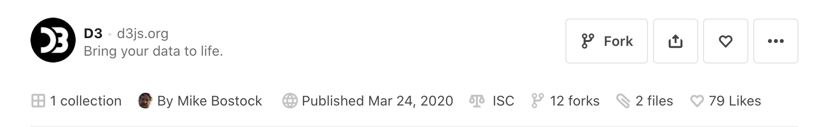
You should check the license of ObservableHQ notebooks before you import them. See the documentation on notebook licenses for additional details on how to do this.

Appendix

```{ojs}
flareData = FileAttachment("examples/flare-2.json").json()
```

```{ojs}
partition = flareData => {
  const root = d3.hierarchy(flareData)
      .sum(d => d.value)
      .sort((a, b) => b.value - a.value);
  return d3.partition()
      .size([2 * Math.PI, root.height + 1])
    (root);
}
```

```{ojs}
color = d3.scaleOrdinal(d3.quantize(d3.interpolateRainbow, flareData.children.length + 1))
```

```{ojs}
format = d3.format(",d")
```

```{ojs}
width = 932
```

```{ojs}
radius = width / 6
```

```{ojs}
arc = d3.arc()
    .startAngle(d => d.x0)
    .endAngle(d => d.x1)
    .padAngle(d => Math.min((d.x1 - d.x0) / 2, 0.005))
    .padRadius(radius * 1.5)
    .innerRadius(d => d.y0 * radius)
    .outerRadius(d => Math.max(d.y0 * radius, d.y1 * radius - 1))
```

```{ojs}
d3 = require("d3@7")
```