Tutorial: Hello, Quarto

Overview

Quarto is a multi-language, next-generation version of R Markdown from Posit and includes dozens of new features and capabilities while at the same being able to render most existing Rmd files without modification.

In this tutorial, we’ll show you how to use RStudio with Quarto. You’ll edit code and markdown in RStudio just as you would with any computational document (e.g., R Markdown) and preview the rendered document in the Viewer tab as you work.

The following is a Quarto document with the extension .qmd (on the left), along with its rendered version as HTML (on the right). You could also choose to render it into other formats like PDF, MS Word, etc.

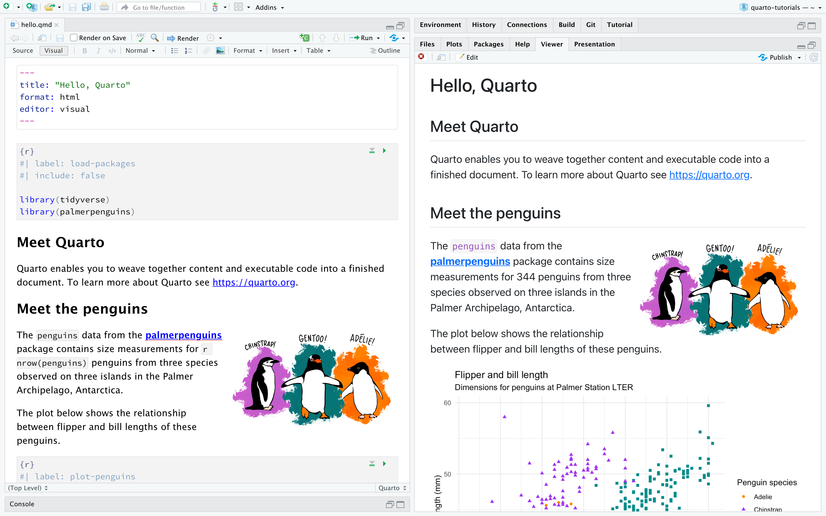
This is the basic model for Quarto publishing—take a source document and render it to a variety of output formats.

If you would like a video introduction to Quarto before you dive into the tutorial, watch the Get Started with Quarto where you can see a preview of authoring a Quarto document with executable code chunks, rendering to multiple formats, including revealjs presentations, creating a website, and publishing on QuartoPub.

If you would like to follow along with this tutorial in your own environment, follow the steps outlined below.

1. Download and install the latest release of RStudio:

   Download RStudio

2. Be sure that you have installed the tidyverse and palmerpenguins packages:

   install.packages("tidyverse")
   install.packages("palmerpenguins")

3. Download the Quarto document (.qmd) below, open it in RStudio, and click on Render.

   Download hello.qmd

Rendering

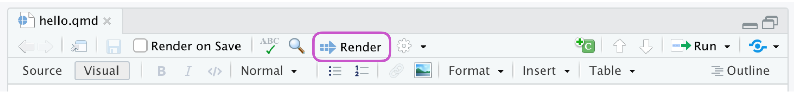
Use the Render button in the RStudio IDE to render the file and preview the output with a single click or keyboard shortcut (⇧⌘K).

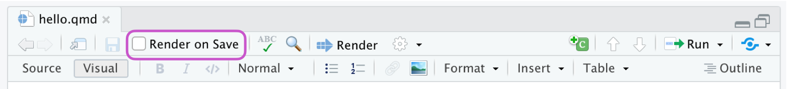
If you prefer to automatically render whenever you save, you can check the Render on Save option on the editor toolbar. The preview will update whenever you re-render the document. Side-by-side preview works for both HTML and PDF outputs.

Note that documents can also be rendered from the R console via the quarto package:

install.packages("quarto")
quarto::quarto_render("hello.qmd")

When rendering, Quarto generates a new file that contains selected text, code, and results from the .qmd file. The new file can be an HTML, PDF, MS Word document, presentation, website, book, interactive document, or other format.

Authoring

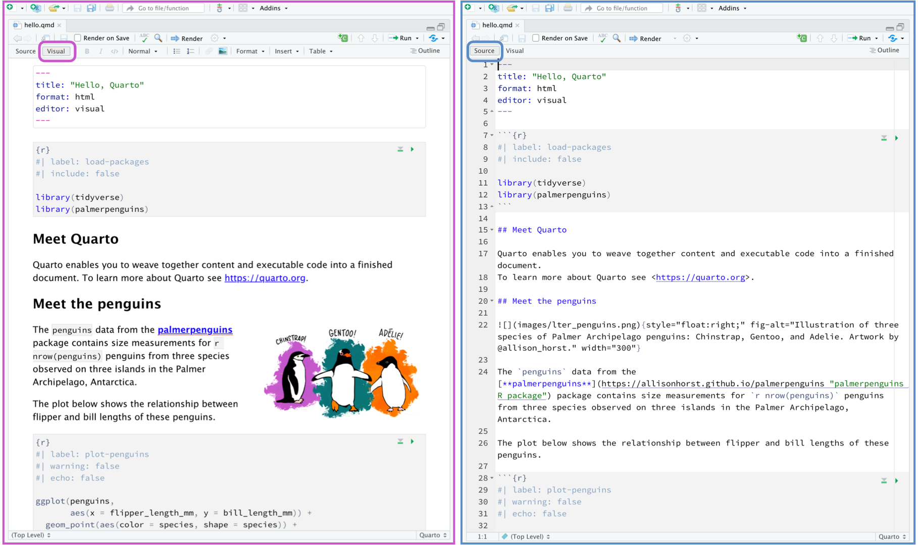
In the image below, we can see the same document in the two modes of the RStudio editor: visual (on the left) and source (on the right). RStudio’s visual editor offers a WYSIWYM authoring experience for markdown. For formatting (e.g., bolding text), you can use the toolbar, a keyboard shortcut (⌘B), or the markdown construct (**bold**). The plain text source code underlying the document is written for you, and you can view/edit it at any point by switching to source mode for editing. You can toggle back and forth between these two modes by clicking on Source and Visual in the editor toolbar (or using the keyboard shortcut ⌘⇧ F4).

Next, let’s turn our attention to the contents of our Quarto document. The file contains three types of content: a YAML header, code chunks, and markdown text.

YAML header

An (optional) YAML header demarcated by three dashes (---) on either end.

---
title: "Hello, Quarto"
format: html
editor: visual
---

When rendered, the title, "Hello, Quarto", will appear at the top of the rendered document with a larger font size than the rest of the document. The other two YAML fields denote that the output should be in html format and the document should open in the visual editor by default.

The basic syntax of YAML uses key-value pairs in the format key: value. Other YAML fields commonly found in headers of documents include metadata like author, subtitle, date as well as customization options like theme, fontcolor, fig-width, etc. You can find out about all available YAML fields for HTML documents here. The available YAML fields vary based on document format, e.g., see here for YAML fields for PDF documents and here for MS Word.

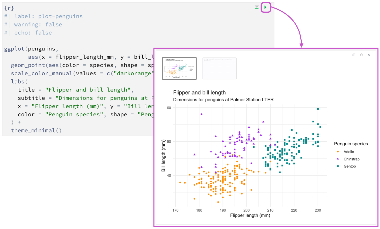
Code chunks

R code chunks identified with {r} with (optional) chunk options, in YAML style, identified by #| at the beginning of the line.

```{r}
#| label: load-packages
#| include: false

library(tidyverse)
library(palmerpenguins)
```

In this case, the label of the code chunk is load-packages, and we set include to false to indicate that we don’t want the chunk itself or any of its outputs in the rendered documents.

In addition to rendering the complete document to view the results of code chunks, you can also run each code chunk interactively in the RStudio editor by clicking the icon or keyboard shortcut (⇧⌘⏎). RStudio executes the code and displays the results either inline within your file or in the Console, depending on your preference.

Markdown text

Text with formatting, including section headers, hyperlinks, an embedded image, and an inline code chunk.

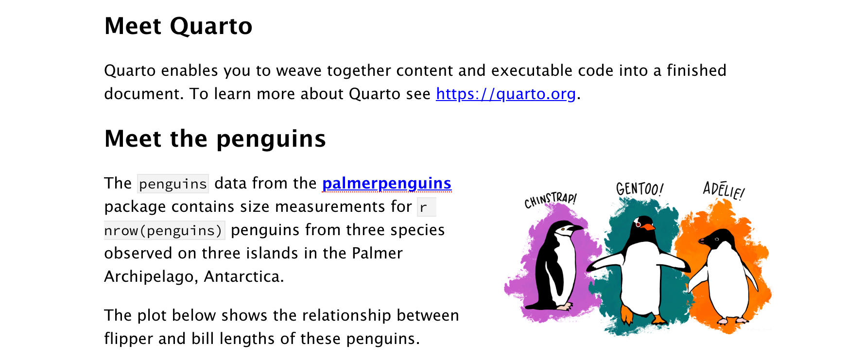
Quarto uses markdown syntax for text. If using the visual editor, you won’t need to learn much markdown syntax for authoring your document, as you can use the menus and shortcuts to add a header, bold text, insert a table, etc. If using the source editor, you can achieve these with markdown expressions like ##, **bold**, etc.

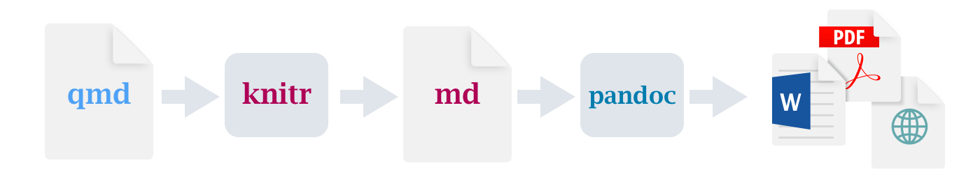
How it works

When you render a Quarto document, first knitr executes all of the code chunks and creates a new markdown (.md) document, which includes the code and its output. The markdown file generated is then processed by pandoc, which creates the finished format. The Render button encapsulates these actions and executes them in the right order for you.

Next Up

You now know the basics of creating and authoring Quarto documents. The following tutorials explore Quarto in more depth:

• Tutorial: Computations — Learn how to tailor the behavior and output of executable code blocks.

• Tutorial: Authoring — Learn more about output formats and technical writing features like citations, crossrefs, and advanced layout.